Tidy Tuesday Visualizations - NY Times Best Sellers

As an avid reader, I was particularly interested in this dataset. I am constantly looking for a new best book to read so this dataset was particularly fun to work with.

Loading Packages / Data

## --- Compiling #TidyTuesday Information for 2022-05-10 ----

## --- There are 2 files available ---

## --- Starting Download ---

## 
## 	Downloading file 1 of 2: `nyt_titles.tsv`
## 	Downloading file 2 of 2: `nyt_full.tsv`

## Warning: One or more parsing issues, call `problems()` on your data frame for details,
## e.g.:
##   dat <- vroom(...)
##   problems(dat)

## --- Download complete ---

## --- Compiling #TidyTuesday Information for 2022-05-10 ----

## --- There are 2 files available ---

## --- Starting Download ---

## 
## 	Downloading file 1 of 2: `nyt_titles.tsv`
## 	Downloading file 2 of 2: `nyt_full.tsv`

## Warning: One or more parsing issues, call `problems()` on your data frame for details,
## e.g.:
##   dat <- vroom(...)
##   problems(dat)

## --- Download complete ---

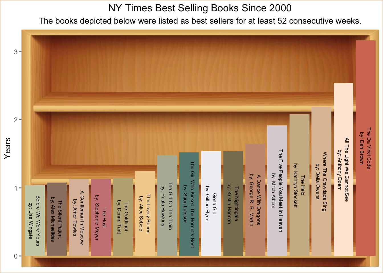
Visualizing Books in the Best Sellers List for 1 Year Since 2000

The Best Sellers list contains books starting in the year 1931 to 2020. I decided to filter the data to only include best sellers from the 21st century. To really get the cream of the crop, I filtered the data again, so that all books included in this analysis were listed as a best seller for at least 52 weeks (1 year).

As shown in the visualization below, the number one bestseller within this time range was The Da Vinci Code by Dan Brown, a book that I still need to read. Of the 16 books listed, my person favorite book that I’ve read thus far, was “The Silent Patient”, there’s nothing better than a good thriller!

# Filtering Data for books that have been best sellers for at least a year

year_bestsellers <- nyt_titles %>%
  filter(total_weeks >= 52) %>%
  filter(year > 2000) %>%
  mutate(total_years  = round(total_weeks / 52, digits = 2)) 

# Clean the titles up:
year_bestsellers$title <- str_to_title(year_bestsellers$title)
year_bestsellers <- year_bestsellers %>% 
  mutate(by_author = paste("by:", author)) %>% 
  mutate(booktitle = paste(title, by_author, sep = "\n"))

img <- readJPEG("test.jpg")
ggplot(year_bestsellers, aes(y = total_years, x = reorder(booktitle, total_years), fill =booktitle)) + 
  background_image(img) + 
  geom_bar(stat = "identity") +
  scale_fill_manual(values = c("#cb997e", "#ddbea9", "#ffe8d6", 
                                "#CDCFb3", "#eff1f3", "#d77a61", 
                               "#dbd3d8", "#b7b7a4", "#648981", 
                               "#bfaf82", "#cfb895", "#CD8485", 
                               "#f1d19b", "#897d5e", "#9C8170", 
                               "#e0c2a5")) + 
  geom_text(aes(label = booktitle), color = "black", size = 2.3, angle = 270, position=position_stack(vjust=0.5)) + 
  labs(y = "Years", x = "", title = "NY Times Best Selling Books Since 2000",
       subtitle = "The books depicted below were listed as best sellers for at least 52 consecutive weeks.") +
  theme(axis.text.x = element_blank(),
        axis.title.x = element_blank(),
        axis.ticks.x = element_blank(), 
        legend.position = "none", 
        plot.title = element_text(hjust = 0.5),
        plot.subtitle = element_text(hjust = 0.5),
        plot.background = element_rect(colour = "#ddbea9"),
  )

Examining Trends in Best Sellers that were Ranked #1 AND were Best Sellers For the Most Weeks that Year

I also examined the books that were ranked #1 for the greatest total number of books for each year. The data was further grouped by what the debut ranking was (i.e., what rank the book received when it first hit the bestsellers list)!

This plot is interactive! Hover over a bar to see the title and author for each top ranked book!

library(plotly)

## 
## Attaching package: 'plotly'

## The following object is masked from 'package:ggplot2':
## 
##     last_plot

## The following object is masked from 'package:stats':
## 
##     filter

## The following object is masked from 'package:graphics':
## 
##     layout

ranked_books <- nyt_titles %>%
  filter(best_rank == 1) %>%
  arrange(desc(total_weeks)) %>%
  group_by(year) %>%
  slice(1) %>% 
  mutate(debut_rank_cat = case_when(
    debut_rank <= 5 ~ "Ranked 1-5", 
    debut_rank > 5 & debut_rank <= 10 ~ "Ranked 5-10",
    debut_rank > 10 & debut_rank <= 15 ~ "Ranked 10-15", 
    TRUE ~ "Ranked 16-20"
  ))
ranked_books$debut_rank <- factor(ranked_books$debut_rank, levels = c("Ranked 1-5", "Ranked 5-10", "Ranked 10-15", "Ranked 16-20"))
ranked_books$title <- str_to_title(ranked_books$title)


p <- ggplot(ranked_books, aes(x = year, y = total_weeks, fill = debut_rank_cat, label1 = title, label2 = author)) + 
  geom_bar(stat = "identity", position = "dodge") + 
  scale_fill_manual(values = c("#796535", "#8d8233", "#da8936", "#d6695a")) +
  labs(title= "#1 Ranked Best Selling Books for Each Year (1931-2020)", y = "Total Weeks as a Best Seller", fill = "What was the book\nranked when\nit first debuted?", y = "Year") + 
  theme(panel.background = element_rect(fill = "white"))

ggplotly(p)

References

[1] Kays R, Dunn RR, Parsons AW, Mcdonald B, Perkins T, Powers S, Shell L, McDonald JL, Cole H, Kikillus H, Woods L, Tindle H, Roetman P (2020) The small home ranges and large local ecological impacts of pet cats. Animal Conservation. doi:10.1111/acv.12563

[2] McDonald JL, Cole H (2020) Data from: The small home ranges and large local ecological impacts of pet cats [United Kingdom]. Movebank Data Repository. doi:10.5441/001/1.pf315732